Polygon Gardens

September 26, 2003
by Jerry McManus

About L-Systems

L-Systems for simulating plant growth

While working on a demo project recently I discovered the wonderful world of Lindenmayer-Systems (L-Systems). L-Systems are string rewriting techniques developed by Astrid Lindenmayer in 1968 that can be used to model the structure of plants.

Iterative string replacement

The basic functionality of an L-System model consists of an initial string called the axiom and a set of production rules which are iteratively applied to that string. The string is examined for single characters which have associated production rules, when a rule is found, the string which corresponds to that character (as defined by the production rule) is substituted into the string. Each successive iteration produces a longer and more complicated string of characters.

Example::
Axiom: F
Rule: F+F-F

Iteration 1:
F+F-F

Iteration 2:
F+F-F + F+F-F - F+F-F

Iteration 3:
F+F-F + F+F-F - F+F-F + F+F-F + F+F-F - F+F-F - F+F-F + F+F-F - F+F-F
And so on...

2d L-Systems

Turtle graphics

In a 2d L-system the final string, after all iterations have been applied, is used as a set of drawing commands to produce a rendering of the plant structure. The drawing commands encoded in the string are used to operate on a cursor, also known as a turtle (from the LOGO programming language), that can be rotated by a given angle and moved along its current heading. For each segment a line is drawn connecting the previous cursor position with the new cursor position.

2d drawing commands:

F	Draw a segment
f	Move cursor without drawing
+	Rotate cursor clockwise by given angle
-	Rotate cursor counter-clockwise by given angle

Example:

Axiom: F
Rule: F+F--F+F

Iteration 1:
F+F--F+F

Iteration 2:
F+F--F+F+F+F--F+F--F+F--F+F+F+F--F+F

Adding branches

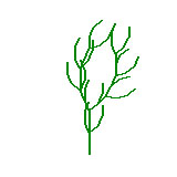
Bracketed L-Systems incorporate the characters '[' and ']' in their production rules to push and pop current branch states from a stack. Utilizing these characters allows the model designer to form structures which branch off of a parent structure without losing the location from which they branch.

Example:

Axiom: F
Rule: FF+[+F-F-F]-[-F+F+F]

Iteration 1:
FF+[+F-F-F]-[-F+F+F]

Iteration 2:
FF+[+F-F-F]-[-F+F+F] FF+[+F-F-F]-[-F+F+F] + [ + FF+[+F-F-F]-[-F+F+F] - FF+[+F-F-F]-[-F+F+F] - FF+[+F-F-F]-[-F+F+F] ] - [ - FF+[+F-F-F]-[-F+F+F] + FF+[+F-F-F]-[-F+F+F] + FF+[+F-F-F]-[-F+F+F] ]

One drawback of this approach is that drawing of the main axis essentially stops while the entire branch is drawn (since it is being drawn in a depth-first fashion). Any interaction which would normally occur between the branch and points higher in the system is impossible.

The process of synchronous branch growth implements the effects of brackets in a different way, producing a breadth-first growth simulation. Instead of placing branches onto a stack, each substring enclosed within brackets is essentially placed in its own object. The objects are placed into a list, each element of which is allowed to perform one rendering command during a given frame. Thus, branch objects can grow simultaneously, which allows for the correct modeling of interaction between branches in the system, such as collision detection between branches.

3d L-systems

3d rotation

True three-dimensional L-Systems can be achieved by replacing the angle property used in a 2d L-System with a set of three-dimensional rotations, one rotation transform for each axis.

3d drawing commands

To encode 3d rotation in the drawing commands the '+' and '-' rotation commands are redefined as 3d rotation on the z-axis and several new characters are added:

+	roll right by the given angle on the z-axis
-	roll left by the given angle on the z-axis
&	pitch forward by the given angle on the x-axis
^	pitch back by the given angle on the x-axis
>	turn right by the given angle on the y-axis
<	turn left by the given angle on the y-axis
\|	turn 180 degrees on the y-axis
!	scale branch by the given percentage

Designing a 3d L-System

Recursive algorithm<

This iterative nature of L-Systems makes the implementation of an L-System ideally suited to a recursive algorithm, as opposed to generating the entire final string first and then rendering it in one pass, left to right. Each time the parser script encounters a character that has an associated production rule it substitutes the rule and then calls itself recursively, passing the rule as the new string to be parsed.

The depth of the recursion is defined by a property that stores the number of iterations to be performed. When the maximum depth is reached the parser switches from applying the production rule and begins drawing branch 'segments' instead.

Nested branches

Because the L-system is parsed recursively, this allows for the branch objects to be 'nested'. Each branch not only stores a list of it's own segments, but it also keeps a list of the child branches that it creates during the recursion. This creates a logical tree structure with parent branches each holding a list of child branches, which in turn hold their own list of child branches, and so on.

Abstraction and presentation

A presentation object is created to parse the list of nested branch objects and create a corresponding 3d object for each segment, in this case a cylinder. The resulting list of 3d objects corresponds to the list of branch objects and has the same tree structure.

In this way the list of 3d branch objects can be operated on independently of the list it was created from. This effectively decouples the abstraction of the L-System from it's presentation, allowing greater flexibility in how the L-System is rendered. For example, the list of 3d objects can be parsed over time to create the effect of animated growth.

The object oriented nature of this system also allows for the 3d branch objects to be easily subclassed into a variety of different forms. Creating, for instance, leaves, buds and flowers as specialized versions of the basic branch.

Our analysis rusults in this object design for our system:

Coding a 3d L-System

3d matrix transforms and matrix multiplication

The basic process for transforming a vector in 3d space is to multiply the vector by a matrix. The 'transform' property in Director is essentially a matrix that is used to multiply the position, scale and rotation vectors of 3d nodes. For our purposes we will use the standard 3 X 3 matrices for rotation transforms which have been defined as follows:

X Rotation Matrix
1	0	0
0	cos(angle)	-sin(angle)
0	sin(angle)	cos(angle)

Y Rotation Matrix
cos(angle)	0	sin(angle)
0	1	0
-sin(angle)	0	cos(angle)

Z Rotation Matrix
cos(angle)	-sin(angle)	0
sin(angle)	cos(angle)	0
0	0	1

The process for applying these 3d rotations in our L-System is to store an angle of rotation (in degrees) for each axis and then multiply the 'up' vector (our direction of growth) by each of the three rotation matrices in succession. This results in a position vector which can be used to place the new segment in 3d space.

This is the code for calculating the position of a new segment:

on mSetPosition(me)

  theVector = vector(0,1,0)

  -->apply x axis rotation matrix
  theAngle = pLAngle * (PI / 180)
  theMatrix = [[1, 0, 0], \
  [0, cos(theAngle), -sin(theAngle)], \
  [0, sin(theAngle), cos(theAngle)]]
  theVector = me.mMultiplyMatrix(theMatrix, theVector)

  -->apply y axis rotation matrix
  theAngle = pUAngle * (PI / 180)
  theMatrix = [[cos(-theAngle), 0, -sin(-theAngle)], \
  [0, 1, 0], \
  [sin(-theAngle), 0, cos(-theAngle)]]
  theVector = me.mMultiplyMatrix(theMatrix, theVector)

  -->apply z axis rotation matrix
  theAngle = pHAngle * (PI / 180)
  theMatrix = [[cos(-theAngle), sin(-theAngle), 0], \
  [-sin(-theAngle), cos(-theAngle), 0], \
  [0, 0, 1]]
  theVector = me.mMultiplyMatrix(theMatrix, theVector)

  -->get new position for given length
  newX = pPosX + pLength * theVector[1]
  newY = pPosY + pLength * theVector[2]
  newZ = pPosZ + pLength * theVector[3]

  return vector(newX, newY, newZ)

end

Model creation, rotation and placement

Once we have our new position and rotation vectors we can store these as properties in a list of branch segments which is then passed to our presentation object for the purpose of creating the actual 3d models.

These are the steps for creating and placing the models:

Create cylinder model
Apply shader
Scale model
Create group node
Translate group to base of cylinder
Add cylinder as child of group
Translate group into position
Rotate group

3d L-System demo

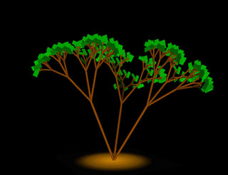
Here is a demo of our 3d L-System with just a few examples of what is possible:

Conclusion

And there you have it, 3d plant life in a polygon garden. On a final note it should be pointed out that L-Systems are not limited to modeling plant structures alone, their iterative nature makes them ideally suited for exploring fractals and other 'self-similar' mathematical models.

You can download the Director source file here.

References

Simulating plant growth
Two-dimensional L-systems
L-System Plant Geometry Generator

Jerry McManus is a freelance Lingo programmer, working and living in Seattle. His love of computer gaming led him to begin his career at Electronic Arts in 1992, eventually working his way up to lead developer on CD-ROM projects beginning with Director 3.0. A recent casualty of The Great Dot Com Crash, Jerry can be found at home working feverishly on any one of several projects including games, books, websites, portfolios, 3d graphics, animations, and a wide variety of other things that somehow never quite seem to get finished...