Raytracing in Lingo: Silly Spheres with Sexy Shadows
February 14, 2001
by Andrew M. Phelps
[Editor's Note: Believe it or not, this article is trimmed down significantly from the original text. The unedited Word document is included with the download files and contains all of the bibliographical references. -DP]
Basic Raytracer Theory and Implementation
Tutorial File Setup
Ray-tracing has now been viable in computer graphics for quite some time, with improvements to renderers happening at the large firms such as Pixar and Alias | Wavefront almost daily, and advanced techniques like motion-blurring and super-sampling quite common. This project implements a simple ray-tracer, and is intended to demonstrate how the theory works. As such, this is essentially a throwback to the ray-tracers of the early 1990s, and it must be noted that it performs like one. Ray-tracing in general, because of the number of calculations involved, is a relatively slow process, and this issue is exacerbated by the fact that Lingo is an interpreted language. Nonetheless, this demo hopefully provides a clear and concise picture of the inner-workings of a rendering system, if not in real time.
The first thing to do is to play with the demo files. Download and uncompress the files into the same directory, open the raytracer.dir file, start the movie, and type the following command in the Message window:
RayTrace(300,300,4,0.75)
Press Enter. After a short amount of time you will see a window pop up labeled Render Window, and it will begin to trace the default scene line by line (referred to in the formal literature as a scanline renderer). The command you gave renders a scene 300 pixels wide, 300 pixels high, with 4 levels of ray reflection, and a 0.75 pixel blur. Note the time it takes on your machine; it is certainly not a real-time engine.
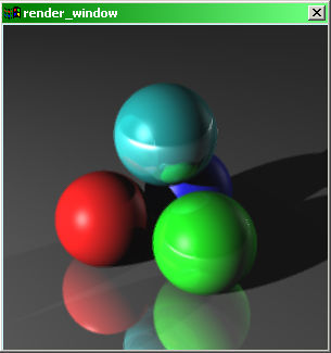
Figure 1. Sample output from raytracer.dir
Basic Mathematical Transforms
The basis of the renderer comes from defining a three-dimensional world. Most of this implementation is based on the discussion of 3D Transforms by R. Stevens (see this and other citations in the downloadable version of this article). While Stevens is implementing in Visual Basic, it is interesting to note that most of the implementations are completely language-independent because they are mathematically based, only the array syntax changes for specifying a matrix.
Essentially this program begins with the basic object of a Point, constructed in the Point3D function under the Matricies script cast member. The other key method in that script is the Mat3Identity function, which creates the classic Identity Matrix. Manipulations and projections of the point then involve using the rest of the functions in the samescript to transform and project the point as needed by the engine. This is accomplished, in essence, by creating the points, creating a matrix, and then using the Mat3Apply or Mat3ApplyFull function depending on whether or not the fourth (scale) value of a point array is 1. If a point has a scale of 1, then it is, by definition, using global world coordinates, if it has a value other than 1, then it needs to be re-expressed using a value of 1 (re-normalized in the commented code), and then transformed.
A number of additional methods are built up in the Matricies script that combine functions to produce the actions common to 3D worlds, namely transform, rotation, and scale. This script also provides the functionality for points to be projected onto a 2D plane, using the Mat3Project function, or, using a wrapper for spherical coordinates, the Mat3PProject function. These, combined with the global variable declarations in the StartMovie script, provide the basis for the world. Most of these functions contain associated comment, where V is an argument of type Point3D, and M is an argument of type Matrix. For a more in-depth explanation of the math involved in creating a world such as this, refer to the references section at the end of the downloadabledocument, as there are countless materials on 3D graphics, matrices, and graphics engines available, many implemented in Lingo already, and for additional documentation and geometric proofs of these precise methods, see Stevens's original derivations.
Scene Objects and Object Heirarchy
The next step in creating the application is the creation of objects in the scene, namely the collection of spheres and the ground plane. Each object is created in a script named ObjName_of_object, so a sphere would be created in ObjSphere, a plane in ObjPlane, etc. Additionally, each of these objects set as its ancestor an object of type ObjGeneric (see Figure 2). This class encapsulates the basic methods for setting attributes for the lighting calculations, and also sets Boolean values for coding clarity with regard to IsReflective and IsTransparent. Each object implements four functions, Initialize, Apply, RayDistance, and HitColor. Initialize should be fairly straightforward; it is called from the DrawData script to instantiate the object. Incidentally, objects are organized on an Objects list, so they can be looped through later. The Apply function takes an argument of type Matrix, and applies that matrix to the coordinates of the object using the Mat3Apply function described earlier. The object stores these transformed coordinates in a separate Point3D object. When the movie is started, the DrawData script is called. In this script, projecting the camera onto the Stage creates a transform matrix, and this transform is then applied to all of the objects in the list.
Figure 2. Object hierarchy of the scene-graph.
Objects are loaded with values to create different colors and effects, according to the following table. Each of these properties is set before the object is added to the list.
Table 1. Attributes of Scene Objects
| Property | Description |
| IsTransparent | Boolean Flag, is the object Transparent? |
| IsReflective | Boolean Flag, is the object Reflective? |
| PSpecN, pKs | Attributes for specular highlights. |
| pHit | X, Y, Z Coordinate data for where an object is hit with a ray. |
| Kdr, Kdg, Kdb | Red, Green and Blue components for diffuse lighting calculation. |
| Kar, Kag, Kab | Red, Green, and Blue components for ambient light calculation. |
| Krr, Krg, Krb | Red, Green, and Blue components for reflected light calculation. |
| Ktr, Ktg, Ktb | Red, Green, and Blue components for transparent light calculation. |
| n1, n2, nt | Constants for reflection and refraction calculations. |
Once these objects exist in their list, and hold their project coordinates, we are ready to move on in creating the rest of the elements necessary to complete the scene, namely the lights and the viewpoint.
Scene Lights and Lighting
The lights in the scene are very simple objects, that hold 2 Point3D values, one for the original coordinates, and one for the coordinates projected by the viewpoint matrix. This is different from many lighting systems that store color and decay information directly within the lights themselves. In the effort of simplicity, this system uses single global values to control much of the light's behavior, namely the ambient values, and the LightKDist value, which is basically a mechanism for how 'bright' the light will appear on object, and how quickly it will fall to shadow. The following table describes the lighting values and their effects on the system.
Table 2. Global Lighting Variables
| Variable | Description |
| LightKdist | Integer describing the fall-off distance of the light. |
| LightIar, LightIab, LightIag | Red,Green,and Blue attributes for ambient light. |
| BackR, BackG, BackB | Red, Green, and Blue components of background color (before applying ambient contribution). |
Cameras and Clipping Planes
There really in essence is not a 'camera' in the sense of most traditional 3D packages. There is simply a viewpoint that is expressed in spherical coordinates, and a matrix that is created from projecting this point onto the 2D viewing plane (in our case, the Render Window). Additionally, it is possible to move the point that the viewpoint is 'looking at' by changing the Focus(X,Y,Z) coordinates. All of the viewpoint variables are set in the startMovie handler; the Projector Matrix is created by calling Mat3Pproject and feeding it the coordinates of the viewpoint, the coordinates of the viewpoint focus, and the nature of the world coordinate system (in this case we are using a 'Y-up' world, where the Y axis points up, the X axis moves across the screen, and the Z axis comes out towards the viewer).
World Creation : Putting It All Together
So in essence these are the parts of the program that are responsible for the creation of the scene and getting the scene to a point that it can be rendered at the desired resolution. All of this occurs without any input from the user of the software, and it occurs in the modules of the program as demonstrated in Figure 3. First, global variables are set that describe the viewpoint and the center of the scene, scene objects are instantiated, as well as light objects, and both objects and lights are held in their respective lists. This occurs inside the DrawData script. All of the objects and lights have their respective coordinates projected and stored in their internal structures as the TransPoint[x] property. Following through the code should be relatively straightforward based on the flowchart and the associated comments in the Lingo scripts. At the end of the completion of the DrawData script, all of the required globals and objects for rendering are ready for rendering, and the movie awaits user input, namely the RayTrace command that you gave when starting the movie.
Figure 3. Flowchart of world creation and startup.
Table 3: Global Viewpoint Variables
| Variable | Description |
| EyeR | The first part of the viewpoint coordinates, expressed in spherical coordinates. This value represents the distance from the origin of the world (set in Focus X, Y and Z). |
| EyePhi | This is the angle between the viewpoint and the XZ plane (assuming a Y-up world, which this is). |
| EyeTheta | The angle representing rotation of the viewpoint around the Y axis. |
| FocusX, FocusY, FocusZ | Point in 3D space that the viewpoint is centered on. . |
| Projector | The Matrix returned by projecting the coordinates above onto the viewing plane. This matrix is then applied to all objects and lights such that when drawn on the plane they appear in proper perspctive. |
The Render Window and Pixel Plotting
Render Window and Lingo Adaptation Technique
Typical ray-tracers have what is called a render window that holds and display the scene as it is being calculated. To emulate that in Director I use a separate Movie In A Window (MIAW). This is a very simple movie, containing only 2 scripts and 1 sprite. The first script is what I consider a standard way to keep a movie running on a single frame, which is the standard go to the frame loop located in the go_frame_loop script. The sprite is a cast member exactly 1 pixel square, and whose single pixelis solid black (R0G0B0).
The third and final script is a method that allows a given pixel to be plotted at a precise RGB value. This is accomplished in Lingo by allowing the script to position the locH and locV of the pixel sprite (in essence placing it on the stage) and setting the RGB color value of this pixel. Because the image size is variable, this movie uses the same sprite over and over again rather than a separate sprite for each pixel. To achieve this illusion, you will notice that the pixel sprite has trails turned on, thus presenting the illusion that we are drawing separate pixels to the render window when in fact we are drawing the same one over and over. The movie starts with the pixel sprite located off the stage:
on plot_pixel x, y, r, g, b
Sprite(1).locH = x
Sprite(1).locV = y
Sprite(1).color = rgb(r,g,b)
updatestage
end
The main rendering loop (called from the RayTrace command you issued at the start of this article) uses a double loop to plot every pixel on in the render view, from left to right, top to bottom. This produces the effect of the image being built line-by-line and is indicative of this generation of ray-tracers, where each pixel value is sampled individually.
The Rendering Loop
The real underlying issue of course, is not looping through the pixels and plotting them but in knowing which color to use. This is finally the intersection of the 3D world with the 2D image plane, and the idea is to some degree a simple one. What this program does in its simplest form is send out rays from the center of projection, through each pixel, and into the scene. The program then checks to see how far into the scene the ray travels, if it reaches an arbitrary infinite value, then it can be assumed that it did not hit anything, and the background should be rendered. If the distance comes back as less than infinite, then the color is calculated based on which object was hit and how that object was lit (see Figure 4).
Figure 4. Basic Ray-Tracing Theory.
This system then, has the added bonus of built-in overlapping and culling of objects, since rays can hit one and only one object first. The process of calculating the ray distance, and the color of an object hit, is exceedingly intensive, and is implemented in the sample file as follows:
For each pixel, a call is made to the RayColor function, which in turn calls the TraceRay function. RayColor is used to average the results from multiple calls to TraceRay, sampling a pixel more than once based on the number of lights in the scene. TraceRay is truly the start of the ray-tracing process, as it loops through each object in the scene, and recursively tries to find the shortest distance by using the RayDistance method of each object on the list. The RayDistance method is built using the classic quadratic for this purpose, derived in full in Foley's master work, implemented by Stevens and many others. The comments in this section of code should explain to some degree the purpose of each calculation.
Once the minimum distance is obtained, and assuming that distance is not infinite, the object that produced the closest intersection with regards to the center of projection is now the active object. The TraceRay function then calls the active object's HitColor routine. HitColor calculates the color of the intersection point. The first step in creating the illusion is tracing a ray from the point of intersection to the light source, and seeing if it gets there without interruption. If it does, then it can be assumed that the light is shining on the surface, if it does not then the surface is in shadow, and as such there should be no diffuse value other than the standard ambient value for the scene. Assuming that the object is lit, the process for diffuse color involves calculating the normal of the surface at the point of intersection, calculating a vector from that point to the light source, then examining the angle of difference between these two vectors. If the angle is large, then the surface faces away from the light and is likely very dim. To measure this, the traditional approach is to take the dot product of the two vectors and multiply them by the base constant of the color of the object, modifying the colors both positively and negatively to produce shading.
The specular highlights found in the system are simply one further step along this idea, using a vector calculated back from to the viewpoint from the point of intersection, and using the dot product of this vector and a vector in the mirror direction to the one described above, multiplied by a constant to determine how 'shiny' the object is. This produces the 'plastic' look common to ray tracing systems before the addition of texture mapping techniques.
Additional Feature Set
Reflection
Reflection is usually the first 'goodie' that people implement in systems such as these, and it is implemented faithfully here. The reason for this is that it is the first logical follow-on to the idea of tracing rays. Essentially, instead of only calculating the color at the point where a ray hits an object, a new ray from that 'hit location' is traced back through the scene to see if it intersects another object. If another object is encountered, that color is calculated and averaged with the first color using a constant that is set to determine how reflective we want the object to look. The greater the constant, the greater the effect of the second color, and thus the less influence the first has. To some degree, this mimics the way light is bent by reflective objects in the real world, and can provide a convincing illusion if the constants and lighting are set at believable levels.
To accomplish this, this program implements a technique often found in graphics systems and more traditional computer science program architecture, but one that this author has rarely used in standard multimedia programming: recursion. The user of this system will pass in the maximum number of times a ray is allowed to 'bounce', referred to as ray-depth. This attribute is passed from the TraceRay function to an object's HitColor method when we calculate the color of an initial ray intersection. The program will then (assuming that the depth is not infinite) reduce this value by 1 and call TraceRay again, this time with a starting location not from the center of projection, but from the last intersection of ray and object. This continues (assuming that none of the rays run to infinity) until the ray-depth value is depleted to zero. Note, that this can drastically effect the overall performance of the system because tuning this value to a high number causes the number of calculations to grow, while there is very little visual effect beyond a relatively low number of recursive iterations. Also note the possibility for 2 perfectly parallel, perfectly reflective planes to trap a ray forever, thus causing an infinite loop, if ray depth is not used.
Transparency and Refraction
The final 'illusion' presented in this demo is that of transparency, with refraction. This is achieved by allowing the ray to pass through the object, and adjusting the angle of the ray based on the inverse normal of the surface and the constants set for the index of refraction. The larger the difference between the first and second constants (n1 and n2) the more the rays will 'bend'.
Pixel Blur and Anti-alias Routines
The Need For Sampling
The need for sampling becomes apparent when considering an original render of the system (see figure 5). In this picture, the edges of the objects are 'popped out' against the scene, producing 'jaggies' along the edges of the objects. This occurs because a single pixel can be one and only one color value, and when calculating the pixels the system must choose weather a pixel lies inside or outside an object. If the edge of the object is at an angle or curves across the pixel grid, this produces the effect seen above, described by Glassner as Spatial Aliasing.
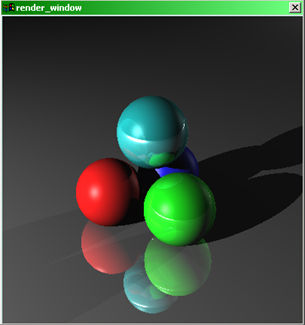
Figure 5: Pre-blur ray-tracer output.
Pixel Blur Routines
The solution to this issue, in its simplest form, is to sample a pixel more than once and then average the results of those samples together to get the final solution. In essence, if the pixel grid is of a finer resolution, then the appearance will be better and the aliasing effects minimized. This solution samples a pixel 5 times, once at its center and 4 times at an offset from the center, one in each direction. This offset is the blur argument passed to the engine at render-time, and should be greater then zero, but not more than one full pixel, otherwise stippling effects will occur.
A sample Director 8 movie and the unedited version of this article (approximately 550K total) is available for download in Mac or Windows format.
Copyright 1997-2026, Director Online. Article content copyright by respective authors.